
Introduction
Both financial institutions and other investors often place significant amounts of money in high-performing credits. These portfolios might contain loans to rather small groups of obligors, for example sovereigns, large corporations or banks. Moreover, credit defaults might be very rare in each one of these groups. Hence, “the law of large numbers” becomes less relevant when it comes to estimating probabilities of default (PD). Values based on some average historical default rate might not be statistically significant enough for prudent investors.
There is however an alternative statistical approach: instead of digressing on straightforward average rates at a given confidence interval, we could put the question “which hypothetical PD would be at the limit of a confidence region, given the observed number of defaults in this particular group of obligors?” This latter approach permits us perform our estimation no matter how few defaults there are. In fact, the method can be applied even if there have been no defaults at all in the portfolio. It also guarantees prudent estimations; either “as is” or adjusted to the portfolios central tendency.
PD estimation for low default portfolios
We will follow a method originally presented by Pluto and Tasche (2005). It requires the assumption that the obligor categories can be ordered correctly in terms of rating grades. That is, if for example there are three rating grades then PDA ≤ PDB ≤ PDC. Furthermore we consider the most prudent possibility, i.e. that all category PDs are equal (and hence equal to the highest, PDC). In the case of independent default events, we can then apply the following equation, which allows for an analytical solution:

where γ is the confidence interval (for example 75%), nA is the number of obligors in group A and r is the total number of defaults (summing all groups). Since we are looking for a boundary value, the lowest PDA that satisfies the equation, we set left-hand side equal to right-hand side and resolve. Notably, the model is valid even if there are no defaults at all, i.e. r = 0.
The estimation for the next rating grade is made by simply excluding the first obligor group (nA) and its related defaults from the equation and resolve for the boundary value of PDB.
In the case of dependent default events, the maths becomes significantly more complex. Nevertheless, it is still possible to build upon the previous model by making the additional assumption that systemic risk affects all assets uniformly, so that there will be a unique value ρ for the correlation between assets. The latter implies that we are actually using a Vasicek one-factor risk model. The PD estimation will then be carried out by finding the expected value for the right-hand side of the following equation, as explained by Benjamin, Cathcart & Ryan (2006):
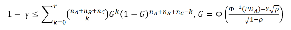
where Y is the single risk factor, to be used in a numerical solution of the equation. Furthermore, Φ and Φ-1 are the standard normal cumulative distribution function and its inverse, respectively.
Monte Carlo simulation in Scala
As mentioned in the previous section, the equation for the case of dependent default events has to be resolved numerically. For this purpose, we have developed a small example programme, written in the Scala language and made available at GitHub. The programme performs a numerical solution via Monte Carlo simulation in the following three steps:
- A pseudorandom sample of values for Y, following a standard normal distribution. The employed sampling algorithm is a Mersenne Twister.
- A map-reduce function that employs each sample value Y in the equation described in the previous section. This allows us to obtain the expected value – i.e. the statistical mean – for a given Y.
- A secant method approximation to resolve for the minimum PD that satisfy the equation and hence becomes our estimated probability of default.
This process is repeated for each group of obligors until all PDs have been obtained. By changing some fixed parameters and the arrays of obligor and default data, most of the results in the reference articles can be replicated. However, the suggested extensions to adjust for portfolio central tendency and to apply a multi-period scenario have not been included in our short programming example.
The Scala programme runs very fast on an ordinary PC or laptop with a sample size of 10,000 Y values. In this case, all results are obtained within a few seconds and are fairly consistent with the figures provided in the reference articles. In order to achieve more reliable results, a sample size of 1,000,000 values might be necessary. Here our estimation takes a couple of minutes per obligor group. Since the secant method approximation needs about ten iterations to reach the solution, we are actually employing the main equation for 1,000,000 samples x 10 iterations x 3 obligor groups = 30,000,000 calculations, which naturally explain the execution times. Anyway, it is of course possible to achieve much faster estimations by distributing the computation among CPU cores or in a cluster.
More information
The Scala programme is available as Open Source code in our GitHub repository: https://github.com/GimleDigital/Scala-Tidbits.
Reference articles:
Pluto, K. and Tasche, D. (2005). Estimating Probabilities of Default for Low Default Portfolios. In B. Engelmann and R. Rauhmeier, Ed., The Basel II Risk Parameters. Berlin: Springer, 2006.
Benjamin, N., Cathcart, A, and Ryan, K. (2006). Low Default Portfolios: A Proposal for conservative Estimation of Default Probabilities. London: Financial Services Authority discussion paper, 2005.
- Log in to post comments